Examine cast data from APL-SURP cruise using a specialized package#
Created for the University of Washington Applied Physics Laboratory’s Summer Undergraduate Research Program (SURP) 2025.
This notebook demonstrates the use of the ctd open-source package to read SeaBird CTD .cnv files and the folium open-source package to create interactive maps of cast locations using information read from the cast files.
This notebook builds off the Quick introduction notebook found on the ctd website.
See the APL-SURP Day 2 notebook to compare the use of the ctd package with operations based solely on the Pandas package. But note that the CTD data file used in that notebook have a somewhat different configuration.
from pathlib import Path

import matplotlib.pyplot as plt
We’ll use the pathlib package (part of the Python Standard Library) to handle file paths more seamlessly via pathlib.Path objects. data_dir is the base directory for the data files. The data files are found on our GitHub repository, under site/notebooks/data/aplsurp_cruises_cnvs_2024
data_dir = Path("./data/aplsurp_cruises_cnvs_2024")
Read a .cnv data file#
We’ll use the Python ctd package to read a .cnv file for one cast, exported directly by the SeaBird software used for managing these data. This file includes data from all sensors (SeaBird CTD and other sensors) as well as metadata about the cruise and the cast, such as location (latitude, longitude and station name), time, sensor names and calibration, etc. The ctd package contains custom functionality for data pre-processing and plotting ocean vertical profiles.
import ctd
cast = ctd.from_cnv(data_dir / "20240718_CTD05_p28.cnv")

type(cast)
pandas.core.frame.DataFrame
The ctd.from_cnv function reads the .cnv file and returns a Pandas DataFrame with custom properties and functions. This DataFrame, cast, contains all “CTD” data collected by sensors during the cast, together with metadata either from each sensor or added to the system software by the operators.
Note that the data goes well beyond conductivity, temperature and depth (pressure), since other sensors are also present.
Examine information about the cast#
Let’s look at the first 5 rows and the DataFrame .info(), to get a feel for the data:
cast.head()
| t090C | sal00 | c0S/m | sbox0Mm/Kg | CStarTr0 | flECO-AFL | ph | par | flag | |
|---|---|---|---|---|---|---|---|---|---|
| Pressure [dbar] | |||||||||
| 6.543 | 14.0140 | 30.7695 | 3.737626 | 225.061 | 68.6557 | 6.8175 | 8.034 | 137.86 | False |
| 6.558 | 14.0138 | 30.7709 | 3.737760 | 224.907 | 68.9782 | 6.8175 | 8.029 | 137.86 | False |
| 6.543 | 14.0135 | 30.7719 | 3.737836 | 224.743 | 69.0319 | 6.8175 | 8.034 | 138.65 | False |
| 6.558 | 14.0134 | 30.7718 | 3.737811 | 224.720 | 69.0050 | 6.8175 | 8.034 | 139.04 | False |
| 6.543 | 14.0128 | 30.7725 | 3.737842 | 224.852 | 68.9782 | 6.8175 | 8.029 | 139.04 | False |
cast.info()
<class 'pandas.core.frame.DataFrame'>
Index: 26928 entries, 6.543 to 1.896
Data columns (total 9 columns):
 #   Column      Non-Null Count  Dtype
---  ------      --------------  -----
 0   t090C       26928 non-null  float64
 1   sal00       26928 non-null  float64
 2   c0S/m       26928 non-null  float64
 3   sbox0Mm/Kg  26928 non-null  float64
 4   CStarTr0    26928 non-null  float64
 5   flECO-AFL   26928 non-null  float64
 6   ph          26928 non-null  float64
 7   par         26928 non-null  float64
 8   flag        26928 non-null  bool
dtypes: bool(1), float64(8)
memory usage: 1.9 MB
The index and columns in this DataFrame show the variables that are read: pressure (the index), temperature, salinity, conductivity, dissolved oxygen concentration, beam transmission, fluorescence, pH, photosynthetically active radiation, and a data quality flag.
The ctd package parses and stores file metadata (from the .cnv header section) in the _metadata property of the DataFrame, for convenient access. This property is a Python dictionary. Let’s look at the raw content.
cast._metadata
{'name': 'C:\\Data\\RC0122ctd\\20240718_CTD05_p28',
 'header': '* Sea-Bird SBE 9 Data File:\n* FileName = C:\\Data\\RC0122ctd\\20240718_CTD05_p28.hex\n* Software Version Seasave V 7.26.7.107\n* Temperature SN = 1121\n* Conductivity SN = 2881\n* Number of Bytes Per Scan = 31\n* Number of Voltage Words = 4\n* Number of Scans Averaged by the Deck Unit = 1\n* System UpLoad Time = Jul 18 2024 08:54:01\n* NMEA Latitude = 47 42.80 N\n* NMEA Longitude = 122 25.16 W\n* NMEA UTC (Time) = Jul 18 2024  15:54:00\n* Store Lat/Lon Data = Append to Every Scan\n* SBE 11plus V 5.2\n* number of scans to average = 1\n* pressure baud rate = 9600\n* NMEA baud rate = 4800\n* GPIB address = 1\n* advance primary conductivity  0.073 seconds\n* advance secondary conductivity  0.073 seconds\n* delete word 3 from scan\n* delete word 4 from scan\n* autorun on power up is disabled\n* S>\n** Ship: R/V Rachel Carson\n** Cruise ID: RC0121\n** Tech: Jalickee\n** Chief Scientist: Boyar\n** Station: p28\n** Cast:  05\n* System UTC = Jul 18 2024 15:54:01\n*END*',
 'config': '# nquan = 10\n# nvalues = 26928\n# units = specified\n# name 0 = depSM: Depth [salt water, m]\n# name 1 = t090C: Temperature [ITS-90, deg C]\n# name 2 = sal00: Salinity, Practical [PSU]\n# name 3 = c0S/m: Conductivity [S/m]\n# name 4 = sbox0Mm/Kg: Oxygen, SBE 43 [umol/kg]\n# name 5 = CStarTr0: Beam Transmission, WET Labs C-Star [%]\n# name 6 = flECO-AFL: Fluorescence, WET Labs ECO-AFL/FL [mg/m^3]\n# name 7 = ph: pH\n# name 8 = par: PAR/Irradiance, Biospherical/Licor\n# name 9 = flag:  0.000e+00\n# span 0 =      0.619,    180.351\n# span 1 =    11.1966,    16.1026\n# span 2 =    29.2562,    30.7725\n# span 3 =   3.442453,   3.755137\n# span 4 =    186.942,    411.365\n# span 5 =    61.9648,    93.5652\n# span 6 =     0.0776,     8.7223\n# span 7 =      7.539,      8.284\n# span 8 = 1.0000e-12, 4.0607e+03\n# span 9 = 0.0000e+00, 0.0000e+00\n# interval = seconds: 0.0416667\n# start_time = Jul 18 2024 15:54:00 [NMEA time, header]\n# bad_flag = -9.990e-29\n# <Sensors count="11" >\n#   <sensor Channel="1" >\n#     <!-- Frequency 0, Temperature -->\n#     <TemperatureSensor SensorID="55" >\n#       <SerialNumber>1121</SerialNumber>\n#       <CalibrationDate>09-Feb-24</CalibrationDate>\n#       <UseG_J>1</UseG_J>\n#       <A>0.00000000e+000</A>\n#       <B>0.00000000e+000</B>\n#       <C>0.00000000e+000</C>\n#       <D>0.00000000e+000</D>\n#       <F0_Old>0.000</F0_Old>\n#       <G>4.80019878e-003</G>\n#       <H>6.69292066e-004</H>\n#       <I>2.48135251e-005</I>\n#       <J>1.91962678e-006</J>\n#       <F0>1000.000</F0>\n#       <Slope>1.00000000</Slope>\n#       <Offset>0.0000</Offset>\n#     </TemperatureSensor>\n#   </sensor>\n#   <sensor Channel="2" >\n#     <!-- Frequency 1, Conductivity -->\n#     <ConductivitySensor SensorID="3" >\n#       <SerialNumber>2881</SerialNumber>\n#       <CalibrationDate>28-Feb-24</CalibrationDate>\n#       <UseG_J>1</UseG_J>\n#       <!-- Cell const and series R are applicable only for wide range sensors. -->\n#       <SeriesR>0.0000</SeriesR>\n#       <CellConst>2000.0000</CellConst>\n#       <ConductivityType>0</ConductivityType>\n#       <Coefficients equation="0" >\n#         <A>0.00000000e+000</A>\n#         <B>0.00000000e+000</B>\n#         <C>0.00000000e+000</C>\n#         <D>0.00000000e+000</D>\n#         <M>0.0</M>\n#         <CPcor>-9.57000000e-008</CPcor>\n#       </Coefficients>\n#       <Coefficients equation="1" >\n#         <G>-1.01388164e+001</G>\n#         <H>1.39630559e+000</H>\n#         <I>-7.42875999e-004</I>\n#         <J>1.21597149e-004</J>\n#         <CPcor>-9.57000000e-008</CPcor>\n#         <CTcor>3.2500e-006</CTcor>\n#         <!-- WBOTC not applicable unless ConductivityType = 1. -->\n#         <WBOTC>0.00000000e+000</WBOTC>\n#       </Coefficients>\n#       <Slope>1.00000000</Slope>\n#       <Offset>0.00000</Offset>\n#     </ConductivitySensor>\n#   </sensor>\n#   <sensor Channel="3" >\n#     <!-- Frequency 2, Pressure, Digiquartz with TC -->\n#     <PressureSensor SensorID="45" >\n#       <SerialNumber>0216</SerialNumber>\n#       <CalibrationDate>11-Jan-24</CalibrationDate>\n#       <C1>-4.562074e+004</C1>\n#       <C2>1.820199e-001</C2>\n#       <C3>1.580430e-002</C3>\n#       <D1>3.615300e-002</D1>\n#       <D2>0.000000e+000</D2>\n#       <T1>3.024088e+001</T1>\n#       <T2>-3.472576e-004</T2>\n#       <T3>4.427560e-006</T3>\n#       <T4>3.763240e-009</T4>\n#       <Slope>0.99989457</Slope>\n#       <Offset>-4.96465</Offset>\n#       <T5>0.000000e+000</T5>\n#       <AD590M>1.176000e-002</AD590M>\n#       <AD590B>-8.544400e+000</AD590B>\n#     </PressureSensor>\n#   </sensor>\n#   <sensor Channel="4" >\n#     <!-- A/D voltage 0, Oxygen, SBE 43 -->\n#     <OxygenSensor SensorID="38" >\n#       <SerialNumber>0023</SerialNumber>\n#       <CalibrationDate>01-Mar-24</CalibrationDate>\n#       <Use2007Equation>1</Use2007Equation>\n#       <CalibrationCoefficients equation="0" >\n#         <!-- Coefficients for Owens-Millard equation. -->\n#         <Boc>0.0000</Boc>\n#         <Soc>0.0000e+000</Soc>\n#         <offset>0.0000</offset>\n#         <Pcor>0.00e+000</Pcor>\n#         <Tcor>0.0000</Tcor>\n#         <Tau>0.0</Tau>\n#       </CalibrationCoefficients>\n#       <CalibrationCoefficients equation="1" >\n#         <!-- Coefficients for Sea-Bird equation - SBE calibration in 2007 and later. -->\n#         <Soc>4.4983e-001</Soc>\n#         <offset>-0.4965</offset>\n#         <A>-3.3116e-003</A>\n#         <B> 1.6506e-004</B>\n#         <C>-2.3831e-006</C>\n#         <D0> 2.5826e+000</D0>\n#         <D1> 1.92634e-004</D1>\n#         <D2>-4.64803e-002</D2>\n#         <E> 3.6000e-002</E>\n#         <Tau20> 1.1400</Tau20>\n#         <H1>-3.3000e-002</H1>\n#         <H2> 5.0000e+003</H2>\n#         <H3> 1.4500e+003</H3>\n#       </CalibrationCoefficients>\n#     </OxygenSensor>\n#   </sensor>\n#   <sensor Channel="5" >\n#     <!-- A/D voltage 1, pH -->\n#     <pH_Sensor SensorID="43" >\n#       <SerialNumber>0929</SerialNumber>\n#       <CalibrationDate>7/8/2024</CalibrationDate>\n#       <Slope>4.5430</Slope>\n#       <Offset>2.8338</Offset>\n#     </pH_Sensor>\n#   </sensor>\n#   <sensor Channel="6" >\n#     <!-- A/D voltage 2, Fluorometer, WET Labs ECO-AFL/FL -->\n#     <FluoroWetlabECO_AFL_FL_Sensor SensorID="20" >\n#       <SerialNumber>FLRTD-8543</SerialNumber>\n#       <CalibrationDate>2023-10-06</CalibrationDate>\n#       <ScaleFactor>6.00000000e+000</ScaleFactor>\n#       <!-- Dark output -->\n#       <Vblank>0.0530</Vblank>\n#     </FluoroWetlabECO_AFL_FL_Sensor>\n#   </sensor>\n#   <sensor Channel="7" >\n#     <!-- A/D voltage 3, Transmissometer, WET Labs C-Star -->\n#     <WET_LabsCStar SensorID="71" >\n#       <SerialNumber>CST-2148</SerialNumber>\n#       <CalibrationDate>2024-04-05</CalibrationDate>\n#       <M>22.0074</M>\n#       <B>-0.1342</B>\n#       <PathLength>0.250</PathLength>\n#     </WET_LabsCStar>\n#   </sensor>\n#   <sensor Channel="8" >\n#     <!-- A/D voltage 4, Altimeter -->\n#     <AltimeterSensor SensorID="0" >\n#       <SerialNumber>1098</SerialNumber>\n#       <CalibrationDate></CalibrationDate>\n#       <ScaleFactor>15.000</ScaleFactor>\n#       <Offset>0.000</Offset>\n#     </AltimeterSensor>\n#   </sensor>\n#   <sensor Channel="9" >\n#     <!-- A/D voltage 5, Free -->\n#   </sensor>\n#   <sensor Channel="10" >\n#     <!-- A/D voltage 6, PAR/Irradiance, Biospherical/Licor -->\n#     <PAR_BiosphericalLicorChelseaSensor SensorID="42" >\n#       <SerialNumber>QSP-2350-70840</SerialNumber>\n#       <CalibrationDate>2023-12-18</CalibrationDate>\n#       <M>1.00000000</M>\n#       <B>0.00000000</B>\n#       <CalibrationConstant>11111111111.11100000</CalibrationConstant>\n#       <Multiplier>1.00000000</Multiplier>\n#       <Offset>-0.90110500</Offset>\n#     </PAR_BiosphericalLicorChelseaSensor>\n#   </sensor>\n#   <sensor Channel="11" >\n#     <!-- A/D voltage 7, Free -->\n#   </sensor>\n# </Sensors>\n# datcnv_date = Jul 19 2024 14:30:42, 7.26.7.129 [datcnv_vars = 9]\n# datcnv_in = C:\\Data\\RC0122ctd\\20240718_CTD05_p28.hex C:\\Data\\RC0122ctd\\20240716_CTD02_P29.XMLCON\n# datcnv_skipover = 0\n# datcnv_ox_hysteresis_correction = yes\n# datcnv_ox_tau_correction = yes\n# file_type = ascii',
 'names': ['depSM',
  't090C',
  'sal00',
  'c0S/m',
  'sbox0Mm/Kg',
  'CStarTr0',
  'flECO-AFL',
  'ph',
  'par',
  'flag'],
 'skiprows': 228,
 'time': datetime.datetime(2024, 7, 18, 22, 54, tzinfo=datetime.timezone.utc),
 'lon': np.float64(-122.41933333333333),
 'lat': np.float64(47.71333333333333)}
Let’s look at the metadata more closely by first examining the dictionary “keys”, then some of the individual items:
metadata = cast._metadata

metadata.keys()
dict_keys(['name', 'header', 'config', 'names', 'skiprows', 'time', 'lon', 'lat'])
We’ll store cast time, latitude and longitude in variables for reuse later in the notebook
metadata['time'], metadata['lat'], metadata['lon']
(datetime.datetime(2024, 7, 18, 22, 54, tzinfo=datetime.timezone.utc),
 np.float64(47.71333333333333),
 np.float64(-122.41933333333333))
print(metadata['header'])
* Sea-Bird SBE 9 Data File:
* FileName = C:\Data\RC0122ctd\20240718_CTD05_p28.hex
* Software Version Seasave V 7.26.7.107
* Temperature SN = 1121
* Conductivity SN = 2881
* Number of Bytes Per Scan = 31
* Number of Voltage Words = 4
* Number of Scans Averaged by the Deck Unit = 1
* System UpLoad Time = Jul 18 2024 08:54:01
* NMEA Latitude = 47 42.80 N
* NMEA Longitude = 122 25.16 W
* NMEA UTC (Time) = Jul 18 2024  15:54:00
* Store Lat/Lon Data = Append to Every Scan
* SBE 11plus V 5.2
* number of scans to average = 1
* pressure baud rate = 9600
* NMEA baud rate = 4800
* GPIB address = 1
* advance primary conductivity  0.073 seconds
* advance secondary conductivity  0.073 seconds
* delete word 3 from scan
* delete word 4 from scan
* autorun on power up is disabled
* S>
** Ship: R/V Rachel Carson
** Cruise ID: RC0121
** Tech: Jalickee
** Chief Scientist: Boyar
** Station: p28
** Cast:  05
* System UTC = Jul 18 2024 15:54:01
*END*
print(metadata['config'])
# nquan = 10
# nvalues = 26928
# units = specified
# name 0 = depSM: Depth [salt water, m]
# name 1 = t090C: Temperature [ITS-90, deg C]
# name 2 = sal00: Salinity, Practical [PSU]
# name 3 = c0S/m: Conductivity [S/m]
# name 4 = sbox0Mm/Kg: Oxygen, SBE 43 [umol/kg]
# name 5 = CStarTr0: Beam Transmission, WET Labs C-Star [%]
# name 6 = flECO-AFL: Fluorescence, WET Labs ECO-AFL/FL [mg/m^3]
# name 7 = ph: pH
# name 8 = par: PAR/Irradiance, Biospherical/Licor
# name 9 = flag:  0.000e+00
# span 0 =      0.619,    180.351
# span 1 =    11.1966,    16.1026
# span 2 =    29.2562,    30.7725
# span 3 =   3.442453,   3.755137
# span 4 =    186.942,    411.365
# span 5 =    61.9648,    93.5652
# span 6 =     0.0776,     8.7223
# span 7 =      7.539,      8.284
# span 8 = 1.0000e-12, 4.0607e+03
# span 9 = 0.0000e+00, 0.0000e+00
# interval = seconds: 0.0416667
# start_time = Jul 18 2024 15:54:00 [NMEA time, header]
# bad_flag = -9.990e-29
# <Sensors count="11" >
#   <sensor Channel="1" >
#     <!-- Frequency 0, Temperature -->
#     <TemperatureSensor SensorID="55" >
#       <SerialNumber>1121</SerialNumber>
#       <CalibrationDate>09-Feb-24</CalibrationDate>
#       <UseG_J>1</UseG_J>
#       <A>0.00000000e+000</A>
#       <B>0.00000000e+000</B>
#       <C>0.00000000e+000</C>
#       <D>0.00000000e+000</D>
#       <F0_Old>0.000</F0_Old>
#       <G>4.80019878e-003</G>
#       <H>6.69292066e-004</H>
#       <I>2.48135251e-005</I>
#       <J>1.91962678e-006</J>
#       <F0>1000.000</F0>
#       <Slope>1.00000000</Slope>
#       <Offset>0.0000</Offset>
#     </TemperatureSensor>
#   </sensor>
#   <sensor Channel="2" >
#     <!-- Frequency 1, Conductivity -->
#     <ConductivitySensor SensorID="3" >
#       <SerialNumber>2881</SerialNumber>
#       <CalibrationDate>28-Feb-24</CalibrationDate>
#       <UseG_J>1</UseG_J>
#       <!-- Cell const and series R are applicable only for wide range sensors. -->
#       <SeriesR>0.0000</SeriesR>
#       <CellConst>2000.0000</CellConst>
#       <ConductivityType>0</ConductivityType>
#       <Coefficients equation="0" >
#         <A>0.00000000e+000</A>
#         <B>0.00000000e+000</B>
#         <C>0.00000000e+000</C>
#         <D>0.00000000e+000</D>
#         <M>0.0</M>
#         <CPcor>-9.57000000e-008</CPcor>
#       </Coefficients>
#       <Coefficients equation="1" >
#         <G>-1.01388164e+001</G>
#         <H>1.39630559e+000</H>
#         <I>-7.42875999e-004</I>
#         <J>1.21597149e-004</J>
#         <CPcor>-9.57000000e-008</CPcor>
#         <CTcor>3.2500e-006</CTcor>
#         <!-- WBOTC not applicable unless ConductivityType = 1. -->
#         <WBOTC>0.00000000e+000</WBOTC>
#       </Coefficients>
#       <Slope>1.00000000</Slope>
#       <Offset>0.00000</Offset>
#     </ConductivitySensor>
#   </sensor>
#   <sensor Channel="3" >
#     <!-- Frequency 2, Pressure, Digiquartz with TC -->
#     <PressureSensor SensorID="45" >
#       <SerialNumber>0216</SerialNumber>
#       <CalibrationDate>11-Jan-24</CalibrationDate>
#       <C1>-4.562074e+004</C1>
#       <C2>1.820199e-001</C2>
#       <C3>1.580430e-002</C3>
#       <D1>3.615300e-002</D1>
#       <D2>0.000000e+000</D2>
#       <T1>3.024088e+001</T1>
#       <T2>-3.472576e-004</T2>
#       <T3>4.427560e-006</T3>
#       <T4>3.763240e-009</T4>
#       <Slope>0.99989457</Slope>
#       <Offset>-4.96465</Offset>
#       <T5>0.000000e+000</T5>
#       <AD590M>1.176000e-002</AD590M>
#       <AD590B>-8.544400e+000</AD590B>
#     </PressureSensor>
#   </sensor>
#   <sensor Channel="4" >
#     <!-- A/D voltage 0, Oxygen, SBE 43 -->
#     <OxygenSensor SensorID="38" >
#       <SerialNumber>0023</SerialNumber>
#       <CalibrationDate>01-Mar-24</CalibrationDate>
#       <Use2007Equation>1</Use2007Equation>
#       <CalibrationCoefficients equation="0" >
#         <!-- Coefficients for Owens-Millard equation. -->
#         <Boc>0.0000</Boc>
#         <Soc>0.0000e+000</Soc>
#         <offset>0.0000</offset>
#         <Pcor>0.00e+000</Pcor>
#         <Tcor>0.0000</Tcor>
#         <Tau>0.0</Tau>
#       </CalibrationCoefficients>
#       <CalibrationCoefficients equation="1" >
#         <!-- Coefficients for Sea-Bird equation - SBE calibration in 2007 and later. -->
#         <Soc>4.4983e-001</Soc>
#         <offset>-0.4965</offset>
#         <A>-3.3116e-003</A>
#         <B> 1.6506e-004</B>
#         <C>-2.3831e-006</C>
#         <D0> 2.5826e+000</D0>
#         <D1> 1.92634e-004</D1>
#         <D2>-4.64803e-002</D2>
#         <E> 3.6000e-002</E>
#         <Tau20> 1.1400</Tau20>
#         <H1>-3.3000e-002</H1>
#         <H2> 5.0000e+003</H2>
#         <H3> 1.4500e+003</H3>
#       </CalibrationCoefficients>
#     </OxygenSensor>
#   </sensor>
#   <sensor Channel="5" >
#     <!-- A/D voltage 1, pH -->
#     <pH_Sensor SensorID="43" >
#       <SerialNumber>0929</SerialNumber>
#       <CalibrationDate>7/8/2024</CalibrationDate>
#       <Slope>4.5430</Slope>
#       <Offset>2.8338</Offset>
#     </pH_Sensor>
#   </sensor>
#   <sensor Channel="6" >
#     <!-- A/D voltage 2, Fluorometer, WET Labs ECO-AFL/FL -->
#     <FluoroWetlabECO_AFL_FL_Sensor SensorID="20" >
#       <SerialNumber>FLRTD-8543</SerialNumber>
#       <CalibrationDate>2023-10-06</CalibrationDate>
#       <ScaleFactor>6.00000000e+000</ScaleFactor>
#       <!-- Dark output -->
#       <Vblank>0.0530</Vblank>
#     </FluoroWetlabECO_AFL_FL_Sensor>
#   </sensor>
#   <sensor Channel="7" >
#     <!-- A/D voltage 3, Transmissometer, WET Labs C-Star -->
#     <WET_LabsCStar SensorID="71" >
#       <SerialNumber>CST-2148</SerialNumber>
#       <CalibrationDate>2024-04-05</CalibrationDate>
#       <M>22.0074</M>
#       <B>-0.1342</B>
#       <PathLength>0.250</PathLength>
#     </WET_LabsCStar>
#   </sensor>
#   <sensor Channel="8" >
#     <!-- A/D voltage 4, Altimeter -->
#     <AltimeterSensor SensorID="0" >
#       <SerialNumber>1098</SerialNumber>
#       <CalibrationDate></CalibrationDate>
#       <ScaleFactor>15.000</ScaleFactor>
#       <Offset>0.000</Offset>
#     </AltimeterSensor>
#   </sensor>
#   <sensor Channel="9" >
#     <!-- A/D voltage 5, Free -->
#   </sensor>
#   <sensor Channel="10" >
#     <!-- A/D voltage 6, PAR/Irradiance, Biospherical/Licor -->
#     <PAR_BiosphericalLicorChelseaSensor SensorID="42" >
#       <SerialNumber>QSP-2350-70840</SerialNumber>
#       <CalibrationDate>2023-12-18</CalibrationDate>
#       <M>1.00000000</M>
#       <B>0.00000000</B>
#       <CalibrationConstant>11111111111.11100000</CalibrationConstant>
#       <Multiplier>1.00000000</Multiplier>
#       <Offset>-0.90110500</Offset>
#     </PAR_BiosphericalLicorChelseaSensor>
#   </sensor>
#   <sensor Channel="11" >
#     <!-- A/D voltage 7, Free -->
#   </sensor>
# </Sensors>
# datcnv_date = Jul 19 2024 14:30:42, 7.26.7.129 [datcnv_vars = 9]
# datcnv_in = C:\Data\RC0122ctd\20240718_CTD05_p28.hex C:\Data\RC0122ctd\20240716_CTD02_P29.XMLCON
# datcnv_skipover = 0
# datcnv_ox_hysteresis_correction = yes
# datcnv_ox_tau_correction = yes
# file_type = ascii
Extract and visualize downcast data only#
The data file contains both “downcast” and “upcast” data, but in this notebook we’ll focus on the downcast data. The ctd package added a .split() function to the cast DataFrame that separates the data into downcast and upcast:
# Separate the data into downcast and upcast
down_cast_df, up_cast_df = cast.split()
cast.info() told us there are 26,928 sets of observations in the file. After splitting and selecting only the downcast, we’re left with 14,921
len(down_cast_df)
14921
We can use the ctd plot_cast function to plot depth profiles of one or more variables. This function has been added to the DataFrame. plot_cast uses plot settings that are tuned to how we typically would visualize depth profiles, so we can get a user-friendly plot very easily.
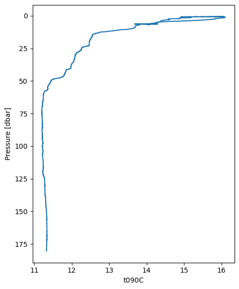
First, let’s do a simple plot of temperature.
down_cast_df["t090C"].plot_cast()
<Axes: xlabel='t090C', ylabel='Pressure [dbar]'>
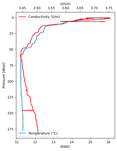
We can also use plot_cast to plot depth profiles of two variables on different axes by using the ax and secondary_y arguments. Note that the raw data is somewhat “noisy”.
ax0 = down_cast_df["t090C"].plot_cast(label="Temperature (°C)")
ax1 = down_cast_df["c0S/m"].plot_cast(
    ax=ax0,
    label="Conductivity (S/m)",
    color="red",
    secondary_y=True,
)

ax0.legend(loc="lower left")
ax1.legend(loc="upper left");
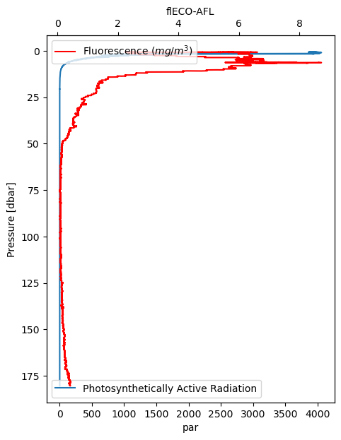
Here are two more variables, both related to light. Fluorescence reflects chlorophyll concentration.
ax0 = down_cast_df["par"].plot_cast(
    label="Photosynthetically Active Radiation")
ax1 = down_cast_df["flECO-AFL"].plot_cast(
    ax=ax0,
    label="Fluorescence ($mg/m^3$)",
    color="red",
    secondary_y=True,
)

ax0.legend(loc="lower left")
ax1.legend(loc="upper left");
Pre-process temperature and conductivity#
We’ve seen that the raw data are somewhat noisy; they contain wiggles and unexpected jumps. Let’s use functions provided by the ctd package to perform data cleaning and pre-processing steps that are typically applied to such data. Note how the functions are “chained” to apply in a sequence, one after the other.
Here, we’ll retain only temperature, conductivity and pressure (pressure is from the DataFrame index).
proc = (
    down_cast_df[["t090C", "c0S/m"]]
    # Remove all data above the water line
    .remove_above_water()
    # Remove all the data above a certain index value, where index can be pressure or depth
    # (it can be unreliable)
    .remove_up_to(idx=4)
    # Remove data spikes
    .despike(n1=2, n2=20, block=100)
    # Apply "low-pass" filter, to remove high-frequency wiggles
    .lp_filter()
    # Remove pressure reversals from the index
    .press_check()
    # Interpolate gaps (this is a Pandas function)
    .interpolate()
    # Bin-average the index (usually pressure) to a given interval (here, 1 meter)
    .bindata(delta=1, method="interpolate")
    # Smooth the data using a window with the requested size
    .smooth(window_len=21, window="hanning")
)

proc.head()
| t090C | c0S/m | |
|---|---|---|
| 7.0 | 13.861522 | 3.605726 |
| 8.0 | 13.695658 | 3.593835 |
| 9.0 | 13.532086 | 3.582112 |
| 10.0 | 13.374312 | 3.570814 |
| 11.0 | 13.225274 | 3.560157 |
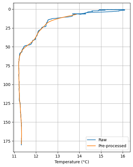
Now let’s compare the raw vs pre-processed temperature:
ax = down_cast_df["t090C"].plot_cast(label="Raw")
proc["t090C"].plot_cast(ax=ax, label="Pre-processed")

ax.grid(True)
ax.legend(loc="lower right")
plt.xlabel("Temperature (°C)");
Map the locations of all casts#
The folium package provides a convenient tool for creating interactive maps. First we’ll map the location of the cast we’ve been examining.
import folium
After initializing a folium map, we add a “marker” with the information about the cast and some plotting configurations
castmap = folium.Map()

folium.Marker(
    location=[metadata['lat'], metadata['lon']],
    icon=folium.Icon(color='red'),
    tooltip="Cruise CTD cast",
    popup=f"Cruise CTD, {metadata['time']}"
).add_to(castmap)

# Set the map extent (bounds) to the extent of the sites
castmap.fit_bounds(castmap.get_bounds())

# Now generate and disply the interactive map
castmap
Because the map shows just one point, it’s zoomed in very closely and the background shows just water. This is an interactive map, so zoom out a few times until you see the Seattle coastline.
Read and map all casts#
Finally, let’s create a map with all the casts. We’ll extract information from the metadata as we did before, but this time we’ll handle even more information in order to generate more extensive (and useful) tooltip and popup information.
get_header_element is a helper function to extract specific metadata values. The next code block loops through all cast .cnv files in the data directory using the pathlib.Path.glob function, reads each cast, extracts the desired metadata, and compiles the casts_metadata list for use in the folium mapping code.
def get_header_element(element_name, metadata):
    """
    Extract the value for the metadata element "element_name"
    from the metadata "header" section
    """
    metadata_header_aslist = metadata['header'].split('\n')
    for e in metadata_header_aslist:
        if element_name in e:
            element_value = e.split(":")[-1].strip()
            return element_value
casts_metadata = []
for cnv_filepath in data_dir.glob("*.cnv"):
    # Read the cast and its metadata
    cast = ctd.from_cnv(cnv_filepath)
    metadata = cast._metadata

    # Let's add additional info to the metadata dictionary,
    # by probing into the cast data and parsing the metadata "header" section
    metadata['depth_max'] = cast.index.max()
    for element_name in ["Cruise ID", "Station", "Cast"]:
        metadata[element_name] = get_header_element(element_name, metadata)

    # Append the metadata to the casts_metadata list
    casts_metadata.append(metadata)
casts_map = folium.Map(tiles='ESRI.OceanBasemap')

# This is just like the single-cast map, except we're now adding
# multiple casts (markers) and populating them with much more information
for castmd in casts_metadata:
    folium.Marker(
        location=[castmd['lat'], castmd['lon']],
        icon=folium.Icon(color='red'),
        tooltip=f"{castmd['Cruise ID']}: {castmd['Station']}-{castmd['Cast']}",
        popup=f"""Cruise {castmd['Cruise ID']}, Station {castmd['Station']},
                Cast {castmd['Cast']}, {castmd['time']:%Y-%m-%d %H:%M},
                Maximum depth {castmd['depth_max']:0.1f} m
                """,
    ).add_to(casts_map)

casts_map.fit_bounds(casts_map.get_bounds())

casts_map