APL SURP Python course - Notebook 4 (completed version)

APL SURP Python course - Notebook 4 (completed version)#

If statements, for loops, xarray, and netCDF files

Created for the University of Washington Applied Physics Laboratory’s Summer Undergraduate Research Program (SURP) 2025.

For additional resources on Python basics, you can consult the following resources on the APL-SURP Python course website:

Tutorials on Python fundamentals: https://uw-apl-surp.github.io/aplsurp-python/overview.html
Complementary lessons on specific Python topics: https://uw-apl-surp.github.io/aplsurp-python/complementary_lessons.html

import numpy as np                         # NumPy is an array and math library
import matplotlib.pyplot as plt            # Matplotlib is a visualization (plotting) library
import pandas as pd                        # Pandas lets us work with spreadsheet (.csv) data
from datetime import datetime, timedelta   # Datetime helps us work with dates and times

import xarray as xr                        # (NEW!) xarray handles multidimensional labeled data

Part 1: `if` statements and `for` loops#

`if` statements#

We can use logical operations to create conditional actions using the if statement.

If the boolean condition evaluates to True, then the lines inside the first block are executed.

Important: note the colons (:) and how the lines below each condition are indented using a Tab or two spaces on your keyboard (you can use a different number of spaces, but they have to be the same within a block).

if <CONDITION #1>:
  <ACTION>
  <ACTION>
  etc.

To create multiple paths for the code to follow, you can use an if-else statement.

If the first condition evaluates to True, then the lines inside the first block are executed.

If the first condition evaluates to False, then Python tests the second elif statement.

If all of the if and elif statements are False, then Python will finally execute the else statement.

if <CONDITION #1>:
  <ACTION>
  <ACTION>
  etc.
elif <CONDITION #2>:  (optional)
  <ACTION>
elif <CONDITION #3>:  (optional)
  <ACTION>
else:                 (optional)
  <ACTION>

First, a quick review of logical operations and booleans. What will these four print statements tell us?

current_temp = 70.0    # 70°F

print(current_temp >= 50)
print(current_temp >= 60)
print(current_temp >= 70)
print(current_temp >= 80)

True
True
True
False

Now, try changing the value of rain_chance below and running the code. Do you understand the control flow?

What range of values for rain_chance will trigger the else statement?

rain_chance = 5    # i.e., a 5% chance of rain

if rain_chance >= 50:
  print('Ugh... I better bring an umbrella.')
elif rain_chance == 0:
  print('I definitely will not need an umbrella.')
elif rain_chance <= 20:
  print('I should be okay without an umbrella.')
else:
  print('I am not sure what to do.')

I should be okay without an umbrella.

`for` loops#

Sometimes, we might want to perform an action multiple times, with small modifications. Coding makes this possible using loops!

A for loop has the following syntax:

for <ELEMENT> in <ITERABLE>:
  <ACTION>
  <ACTION>
  etc.

Here, <ITERABLE> can be a list, array, string, or other collection of elements. You can give <ELEMENT> any unique variable name, and that variable will typically only be used inside the loop.

Run and consider the following examples:

countdown = [4,3,2,1]

for item in countdown:
  print(item)

for character in 'floats':
  print(character)

f
l
o
a
t
s

for num in np.arange(0,7,2):
  print(num)

# These are the monthly average temperatures for Seattle from before
seattle_temps = np.array([40.0,40.6,44.2,48.4,54.9,60.2,66.2,66.7,60.5,52.0,44.5,39.6])

# This loop counts the number of months in which temps are warmer than 60°F:
warm_months = 0

for month in np.arange(0,12):
  this_month_temp = seattle_temps[month]
  if this_month_temp > 60.0:
    warm_months = warm_months + 1

print(f'On average, there are {warm_months} warm months in Seattle!')

On average, there are 4 warm months in Seattle!

You already learned how to calculate the sum of an array of numbers using np.sum().

Now, try to calculate the average Seattle annual temperature by writing a for loop below. There are at least two different ways to write the loop!

# You can reuse the variable "seattle_temps" defined earlier

# Write your code below:

# Option 1:
sum_temp = 0
for temp in seattle_temps:
  sum_temp += temp

# Option 2:
sum_temp = 0
for index in np.arange(len(seattle_temps)):
  sum_temp += seattle_temps[index]

# Finally, print the average temperature by adding it to the print() statement:
print(f'The average annual temperature is: {sum_temp / len(seattle_temps):.2f} °F')
# Here we give equal weight to every month, so this isn't fully accurate

The average annual temperature is: 51.48 °F

Note: Numpy arrays and Pandas DataFrames provide capabilities that often make the use of if and for statements unnecessary. Logical operations can generate boolean indices applied over arrays, and functions can be applied over all elements in an array or column.

Part 2: `xarray` and netCDF files#

Intro to netCDF files#

We’ve been working with NumPy arrays, and we know that they have axes. A 3-D array, for instance, has 3 axes. NumPy calls them axes 0, 1, and 2, but you could also think of them as x, y, and z, or longitude, latitude, and depth. And we know from indexing that we can identify a value by its coordinates along those axes.

NumPy arrays.png

Image source: digitalearthafrica.org

You will often find multidimensional data is from climate or weather models, satellite products, and anything else that can be shown on a map.

In these data sets, Earth is often divided into grid cells in order to simplify the challenge of mapping parameters like ocean temperature or cloud cover all around the world.

As the image below shows, those grid cells often extend in both the horizontal dimension (latitude and longitude) as well as the vertical dimension (height, or depth).

Image source: Caltech

xarray is an important community-developed package that lets us work with gridded data.

In science, gridded data is generally provided using netCDF files, which will usually (but not always) have the file extension .nc.

Because netCDF files are compressed, you can’t simply open them on your computer in TextEdit or Notepad or Excel or Google Sheets. Most of the time, we have to write code to look inside them.

Image source: Matthew Rocklin

The image above is what you might see when you open a netCDF file in xarray. The file may contain multiple variables: in this example, temperature, pressure, elevation, and land_cover.

Those variables will be aligned along a few dimensions — in this case, latitude, longitude, and time.

But not every variable will use all the dimensions. Here, temperature is 3-D, while elevation is only 2-D, because the land elevation doesn’t change much over time (at least over human time scales!).

The dimensions themselves will have coordinates, which are the indices with numbers that let you locate a certain data value along a dimension. A set of coordinates might be: latitude = 70°N, longitude = 130°W (which is the same as -130°E), and time = datetime(2025,7,24).

Lastly, netCDF files have attributes, which are just simple pieces of text (or “metadata”) that may describe how the data set was created, the version of the data set, the units of variables, and other useful info.

Plotting data from xarray#

Just like Pandas, xarray comes with built-in plotting functions that are similar to those in Matplotlib.

You can usually add .plot() after an xarray 1-D or 2-D variable to create a simple plot.

For example, let’s plot the chlorophyll on the most recent day of data:

# Create a quick plot
ds['chla'].isel(time=-1).plot()

<matplotlib.collections.QuadMesh at 0x7d7c7ec5ef50>

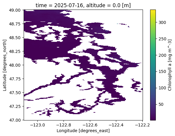
../_images/71605f323d689c544aa1e09c32bad2518ca53328b591c0362fbfd397d85f9163.png

Notice that the color range seems to be too big. Most of the data has much lower chlorophyll values!

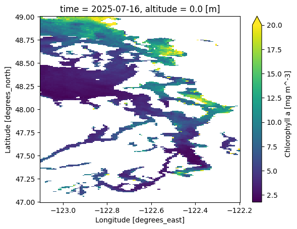
Let’s set the color range to have a maximum value of 20 mg/m^3 using the vmax argument.

Can you find Seattle on this map of Puget Sound?

# Specify the maximum color range
ds['chla'].isel(time=-1).plot(vmax=20.0)

<matplotlib.collections.QuadMesh at 0x7d7c7e9eecd0>

../_images/3044c1126f437a5e13407b2066af52af4b8bb7e21fac896d4641523a8026ee57.png

Just like NumPy arrays or Pandas DataFrames and Series, you can do math using xarray objects!

The beauty of xarray is that it will align coordinates to make sure the right values are being added, subtracted, multiplied, or divided.

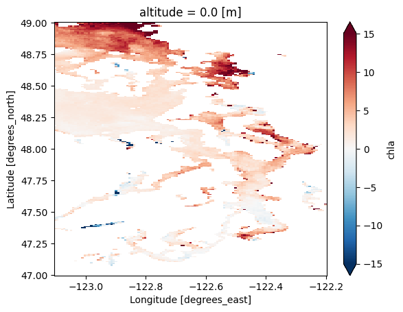
Can you calculate how chlorophyll has changed between the first day of data and the most recent day of data, then create a plot of the change?

# Write your code here:
chl_diff = ds['chla'].isel(time=-1) - ds['chla'].isel(time=0)
chl_diff.plot(robust=True)

# Note that adding "robust=True" inside .plot() removes outlier points outside the
#   2nd and 98th percentiles, making it easier to visualize the data.

# We could also write:
# chl_diff.plot(vmin=-15,vmax=15,cmap='RdBu_r')

<matplotlib.collections.QuadMesh at 0x7d7c7a1a5150>

../_images/d0632fc2563e55baec306c925eccd015d23e2df1a06fd41de2489aa2bbbd737a.png

Manipulating xarray data#

Similar to Pandas, you can apply NumPy functions like .mean() to an xarray object.

For example, we can calculate the average across the longitude dimension—in other words, across all longitudes. That leaves time, latitude, and altitude as the remaining dimensions:

data.mean(dim='longitude')

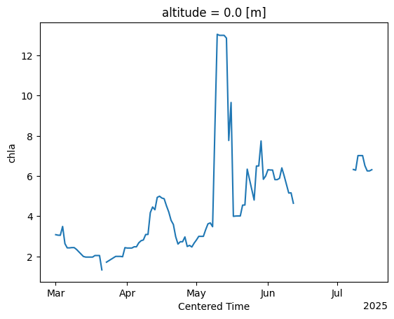
Let’s calculate the average chlorophyll over time within the central Puget Sound region. Here we’ll specify two dimensions inside .mean(): latitude and longitude.

Notice how these operations form a chain:

Variable selection, then
Coordinate selection/slicing, then
Dimension reduction (averaging), then
Finally, plotting!

ds['chla'].sel(longitude=slice(-122.55,-122.3),
               latitude=slice(48,47.50)).mean(dim=['longitude',
                                                   'latitude']).plot()

[<matplotlib.lines.Line2D at 0x7d7c79d8f590>]

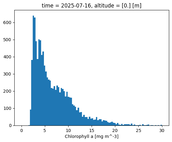
../_images/4ed7f1533215d9b061ef27f1d9457b5a77df83f4c2df687f551e4e19cf6c48e7.png

Another neat quick plotting option is the histogram, .plot.hist(), which shows the distribution of chlorophyll values within specified bins:

ds['chla'].isel(time=-1).plot.hist(bins=100,range=[0,30]);

../_images/f52f91da73dbd58d82759ea903b3ecda01d13feb8ec6aa2dbf0d922395392206.png

APL SURP Python course - Notebook 4 (completed version)

Contents

APL SURP Python course - Notebook 4 (completed version)#

Part 1: `if` statements and `for` loops#

`if` statements#

`for` loops#

Part 2: `xarray` and netCDF files#

Intro to netCDF files#

Intro to xarray#

Selecting data in xarray#

Plotting data from xarray#

Manipulating xarray data#

APL SURP Python course - Notebook 4 (completed version)

Contents

APL SURP Python course - Notebook 4 (completed version)#

Part 1: if statements and for loops#

if statements#

for loops#

Part 2: xarray and netCDF files#

Intro to netCDF files#

Intro to xarray#

Selecting data in xarray#

Plotting data from xarray#

Manipulating xarray data#

Part 1: `if` statements and `for` loops#

`if` statements#

`for` loops#

Part 2: `xarray` and netCDF files#