APL SURP Python course - Notebook 3 (completed version)

Line and scatter plots, depth profiles, timeseries data, logical operations, if statements and for loops and more

Created for the University of Washington Applied Physics Laboratory’s Summer Undergraduate Research Program (SURP) 2025.

For additional resources on Python basics, you can consult the following resources on the APL-SURP Python course website:

• Tutorials on Python fundamentals: https://uw-apl-surp.github.io/aplsurp-python/overview.html

• Complementary lessons on specific Python topics: https://uw-apl-surp.github.io/aplsurp-python/complementary_lessons.html

import numpy as np                         # NumPy is an array and math library
import matplotlib.pyplot as plt            # Matplotlib is a visualization (plotting) library
import pandas as pd                        # Pandas lets us work with spreadsheet (.csv) data
from datetime import datetime, timedelta   # Datetime helps us work with dates and times

Part 1: Line and scatter plots

It’s time for us to start creating visualizations of data, called plots.

At the top of this page, we imported the package Matplotlib using:

import matplotlib.pyplot as plt

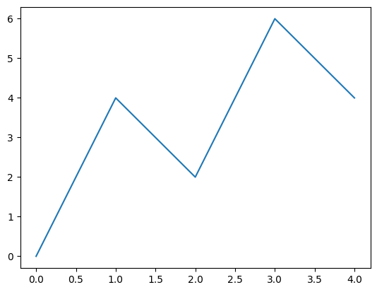
Creating a line plot is simple. We use the Matplotlib function plt.plot(). The basic form of the function is:

plt.plot(X, Y, <FORMAT_ARGUMENTS>...)

Here, X and Y should be 1-D lists or arrays of data. The options for <FORMAT_ARGUMENTS> can be found on Matplotlib’s documentation webpage.

x = np.array([0,1,2,3,4])
y = np.array([0,4,2,6,4])

plt.plot(x,y)

[<matplotlib.lines.Line2D at 0x79200e81f750>]

Some formatting arguments include:

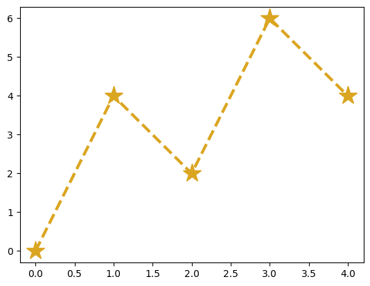
• c or color: line color (options: 'k' or 'black' for black, 'red' for red, etc. – see this page for color options)

• lw or linewidth: line width (a number; the default is 1.5)

• ls or linestyle: line style (options: '-', '--', '-.', ':')

• marker: optional marker style (options: '.', 'o', 'v', '^', '<', '>', 's', '*', etc.)

• ms or markersize: optional marker size (a number)

Try plotting x versus y again, except this time use a “goldenrod”-colored dashed line of width 2.5 with star-shaped markers of size 20:

# Write your code here:
plt.plot(x, y, color='goldenrod', lw=3, ls='--', marker='*', ms=20)

[<matplotlib.lines.Line2D at 0x791ff8b4e010>]

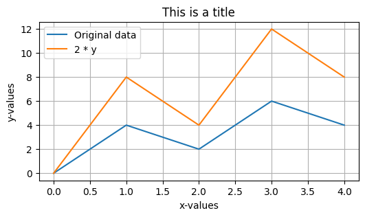
Some other options include changing the figure size by starting with a call to:

plt.figure(figsize=(WIDTH,HEIGHT))

Adding x-axis and y-axis labels and a title at the top:

plt.xlabel(STRING)

plt.ylabel(STRING)

plt.title(STRING)

Adding grid lines using:

plt.grid()

Or adding a plot legend by specifying the label argument in plt.plot() and adding using:

plt.legend()

Check out these additional formatting options below:

plt.figure(figsize=(6,3))
plt.plot(x, y, label='Original data')
plt.plot(x, 2*y, label='2 * y')   # y-values are multiplied by 2 here
plt.legend()
plt.grid()
plt.xlabel('x-values')
plt.ylabel('y-values')
plt.title('This is a title');

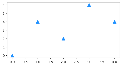
We can also create a scatter plot with just the points (no line). The function is similar to plt.plot():

plt.scatter(X, Y, s=SIZE, c=COLOR, marker=MARKER_STYLE, etc.)

plt.figure(figsize=(6,3))
plt.scatter(x, y, s=100, c='dodgerblue', marker='^');

---

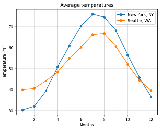
Let’s bring it all together! Below, try plotting the monthly temperatures in New York, NY and Seattle, WA. Use line plots with circle-shaped markers (or add scatter points separately). Include a legend and label the plot appropriately.

# Monthly temperatures in °F
temp = np.array([
    [30.3,32.0,39.4,50.8,60.9,70.3,76.0,74.5,68.1,56.6,45.8,36.5],  # New York
    [40.0,40.6,44.2,48.4,54.9,60.2,66.2,66.7,60.5,52.0,44.5,39.6]   # Seattle
])

# Write your code below:
months = np.arange(1,13)
plt.plot(months, temp[0,:], marker='o', label='New York, NY')
plt.plot(months, temp[1,:], marker='o', label='Seattle, WA')
plt.legend()
plt.xlabel('Months')
plt.ylabel('Temperature (°F)')
plt.title('Average temperatures')
plt.grid()

R/V Rachel Carson CTD depth profiles

Image source: Emilio Mayorga, DINO SIP (SURP predecessor) 2024 cruise

First, let’s download two .csv data files from Google Drive here (we already used the two Rachel Carson files in the previous notebook!). Each file is a conductivity-temperature-depth (CTD) cast that was collected from the ship R/V Rachel Carson off of Carkeek Park near Seattle. There are 4 csv files on that folders; go ahead and save all 4 to your computer.

Next, we can upload the files to this Google Colab notebook. Click the sidebar folder icon on the left, then use the page-with-arrow icon at the top to select the files and upload them.

Note that uploaded files will be deleted from Google Colab when you refresh this notebook!

We will specify each filepath using string variables:

Now, let’s plot the ocean CTD profiles measured by the R/V Rachel Carson. First we’ll read the two CTD csv files using pandas read_csv, as we did in the previous notebook.

Let’s remind ourselves of what the pandas DataFrame looks like:

filepath_1 = '/content/2023051001001_Carkeek.csv'
filepath_2 = '/content/2023051101001_Carkeek.csv'

data_1 = pd.read_csv(filepath_1, comment='#')
data_2 = pd.read_csv(filepath_2, comment='#')

# Note: in a notebook, we don't actually need the "display()" function
# to print out a variable (including a DataFrame) with nice formatting
data_1

	Unnamed: 0	index	altM	CStarTr0	c0mS/cm	density00	depSM	latitude	longitude	flECO-AFL	...	sbeox0Mg/L	sbeox0ML/L	ph	potemp090C	prDM	sal00	t090C	scan	nbf	flag
0	0	3407	98.53	71.0825	31.662958	1021.7317	2.101	47.71418	-122.40854	2.8127	...	10.6450	7.4488	9.271	10.2155	2.119	28.3385	10.2157	3408	0	0.0
1	1	3408	98.53	71.0825	31.662061	1021.7317	2.005	47.71418	-122.40854	2.8127	...	10.6446	7.4484	9.271	10.2140	2.022	28.3388	10.2143	3409	0	0.0
2	2	3409	98.53	71.0825	31.661464	1021.7323	2.045	47.71418	-122.40854	2.8127	...	10.6443	7.4483	9.271	10.2129	2.062	28.3391	10.2131	3410	0	0.0
3	3	3410	98.53	71.0825	31.660448	1021.7323	2.005	47.71418	-122.40854	2.8713	...	10.6441	7.4481	9.271	10.2117	2.022	28.3390	10.2119	3411	0	0.0
4	4	3411	98.53	71.0825	31.658416	1021.7325	1.981	47.71418	-122.40854	3.1057	...	10.6443	7.4483	9.271	10.2093	1.998	28.3389	10.2095	3412	0	0.0
...	...	...	...	...	...	...	...	...	...	...	...	...	...	...	...	...	...	...	...	...	...
8200	8200	11607	11.99	83.1087	31.920640	1024.1134	173.726	47.71316	-122.40812	0.1753	...	7.0198	4.9120	8.788	8.3719	175.266	30.0190	8.3887	11608	0	0.0
8201	8201	11608	11.99	83.1087	31.920640	1024.1135	173.726	47.71316	-122.40812	0.1753	...	7.0201	4.9123	8.788	8.3717	175.266	30.0191	8.3886	11609	0	0.0
8202	8202	11609	11.99	83.1087	31.920820	1024.1141	173.846	47.71316	-122.40812	0.1753	...	7.0204	4.9125	8.788	8.3718	175.387	30.0191	8.3887	11610	0	0.0
8203	8203	11610	11.99	83.1087	31.920579	1024.1129	173.613	47.71316	-122.40812	0.1753	...	7.0205	4.9125	8.783	8.3719	175.152	30.0190	8.3887	11611	0	0.0
8204	8204	11611	11.99	83.1087	31.920340	1024.1135	173.846	47.71316	-122.40812	0.1753	...	7.0209	4.9128	8.788	8.3720	175.387	30.0184	8.3889	11612	0	0.0

8205 rows × 21 columns

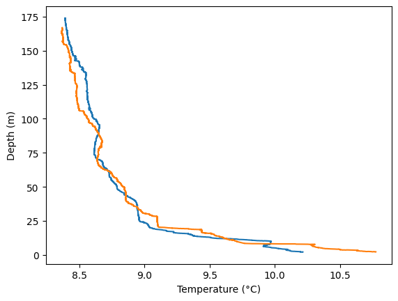
With the tools we have, we can make line plots of temperature vs. depth that include both CTD casts.

In the code below, we explicitly label the x- and y- axes.

plt.plot(data_1['t090C'], data_1['depSM'])
plt.plot(data_2['t090C'], data_2['depSM'])
plt.xlabel('Temperature (°C)')
plt.ylabel('Depth (m)')

Text(0, 0.5, 'Depth (m)')

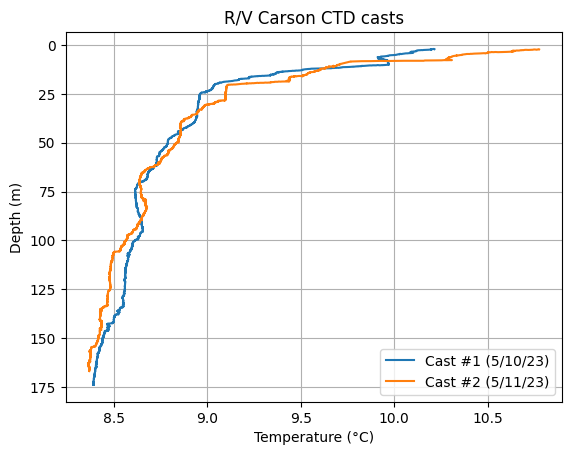
Hmm, it’d be more intuitive to have depth increasing from 0 at the top (the surface); and more useful to add a legend that clarifies which cast is which, a plot title and a grid.

# Temperature vs. depth profile
plt.plot(data_1['t090C'], data_1['depSM'], label='Cast #1 (5/10/23)')
plt.plot(data_2['t090C'], data_2['depSM'], label='Cast #2 (5/11/23)')
plt.xlabel('Temperature (°C)')
plt.ylabel('Depth (m)')

plt.title('R/V Carson CTD casts')
plt.legend()
plt.gca().invert_yaxis()  # This reverses the y-axis. gca stands for "get current axes"
plt.grid()

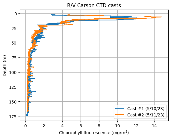
Can you try plotting another parameter vs. depth? Note: the file contains salinity (sal00), oxygen (sbeox0Mg/L), chlorophyll fluorescence (flECO-AFL), and pH (ph) data.

# Write your code here:
plt.figure()
plt.plot(data_1['flECO-AFL'], data_1['depSM'], label='Cast #1 (5/10/23)')
plt.plot(data_2['flECO-AFL'], data_2['depSM'], label='Cast #2 (5/11/23)')
plt.xlabel('Chlorophyll fluorescence (mg/m$^3$)')
plt.ylabel('Depth (m)')
plt.legend()
plt.gca().invert_yaxis()   # This reverses the y-axis
plt.title('R/V Carson CTD casts')
plt.grid()

Part 2. Exploring ocean time series data from the Seattle Aquarium

Seattle is located in King County. King County’s Department of Natural Resources & Parks maintains several ocean measurement stations in Puget Sound. These sensors monitor the water quality and ocean conditions.

One of these stations is at the Seattle Aquarium on the waterfront in downtown Seattle. The station consists of a mooring with two sensors. Sensor #1 is at a depth of 1 meter, and sensor #2 is at a depth of 10 m.

The mooring data can be obtained from King County here: https://green2.kingcounty.gov/marine-buoy/Data.aspx. However, the data requires a bit of processing before it can be loaded into Python. The data can also be conveniently visualized on the NANOOS Visualization System Data Explorer, here.

You can download the processed data file from Google Drive here. This CSV file, SeattleAquarium_7_2_2025_to_7_15_2025.csv, contains data measured every 15 minutes for the two weeks from July 2 to July 15, 2025.

Image source: MyEdmondsNews

The following call to pd.read_csv() will load the data file correctly.

The function arguments will ignore comments (comment='*'), set the header to the first non-commented row (header=0), set the index to the first column (index_col=0), interpret that column as datetimes (parse_dates=True), and specify the file input encoding (encoding='unicode_escape').

# Run this code to load the data
# When a function uses many arguments, it can be convenient for readability
# to specify each argument assignment in one line, like this:
aqua = pd.read_csv(
    '/content/SeattleAquarium_7_2_2025_to_7_15_2025.csv',
    comment='*',
    header=0,
    index_col=0,
    parse_dates=True,
    encoding='unicode_escape'
)

# .head(n) displays the first n records, where the default is n=5
# .tail(n) diplays the last n records.
aqua.head()

/tmp/ipython-input-2993415281.py:4: UserWarning: Could not infer format, so each element will be parsed individually, falling back to `dateutil`. To ensure parsing is consistent and as-expected, please specify a format.
  aqua = pd.read_csv(

	1_Depth_m	Qual_1_Depth	2_Depth_m	Qual_2_Depth	1_Water_Temperature_degC	Qual_1_Water_Temperature	2_Water_Temperature_degC	Qual_2_Water_Temperature	1_Salinity_PSU	Qual_1_Salinity	...	Qual_2_Sonde_pH	1_Density_kg/m^3	Qual_1_Water_Density	2_Density_kg/m^3	Qual_2_Water_Density	1_Sonde_Batt_V	2_Sonde_Batt_V	Logger_Batt_V	1_Sonde_ID	2_Sonde_ID
Date
2025-07-02 00:00:00	0.852	210	9.799	210	13.415	210	11.443	210	29.021	210	...	210	1021.68965	210	1022.65046	210	11.9	13.8	13.1	NaN	NaN
2025-07-02 00:15:00	0.845	210	9.769	210	13.636	210	11.456	210	28.910	210	...	210	1021.56106	210	1022.63347	210	11.9	13.8	13.1	NaN	NaN
2025-07-02 00:30:00	0.844	210	9.791	210	13.356	210	11.447	210	29.042	210	...	210	1021.71730	210	1022.63654	210	11.9	13.8	13.1	NaN	NaN
2025-07-02 00:45:00	0.865	210	9.811	210	13.274	210	11.422	210	29.080	210	...	210	1021.76240	210	1022.65867	210	11.9	13.8	13.1	NaN	NaN
2025-07-02 01:00:00	0.846	210	9.823	210	13.298	210	11.390	210	29.061	210	...	210	1021.74305	210	1022.67361	210	11.9	13.8	13.1	NaN	NaN

5 rows × 39 columns

Since Pandas won’t display all the column names (there are too many!), we can use the .columns attribute to see them:

# Note: we don't need "print()" or "display()" ;)
aqua.columns

Index(['1_Depth_m', 'Qual_1_Depth', '2_Depth_m', 'Qual_2_Depth',
       '1_Water_Temperature_degC', 'Qual_1_Water_Temperature',
       '2_Water_Temperature_degC', 'Qual_2_Water_Temperature',
       '1_Salinity_PSU', 'Qual_1_Salinity', '2_Salinity_PSU',
       'Qual_2_Salinity', '1_Dissolved_Oxygen_%Sat', '1_Dissolved_Oxygen_mg/L',
       'Qual_1_DO', '2_Dissolved_Oxygen_%Sat', '2_Dissolved_Oxygen_mg/L',
       'Qual_2_DO', '1_Chlorophyll_Fluorescence_ug/L',
       'Qual_1_Chlorophyll_Fluorescence', '2_Chlorophyll_Fluorescence_ug/L',
       'Qual_2_Chlorophyll_Fluorescence', '1_Turbidity_NTU',
       'Qual_1_Turbidity', '2_Turbidity_NTU', 'Qual_2_Turbidity', '1_Sonde_pH',
       'Qual_1_Sonde_pH', '2_Sonde_pH', 'Qual_2_Sonde_pH', '1_Density_kg/m^3',
       'Qual_1_Water_Density', '2_Density_kg/m^3', 'Qual_2_Water_Density',
       '1_Sonde_Batt_V', '2_Sonde_Batt_V', 'Logger_Batt_V', '1_Sonde_ID',
       '2_Sonde_ID'],
      dtype='object')

We can also call .info() to get even more information about the DataFrame in a nicely formatted presentation:

aqua.info()

<class 'pandas.core.frame.DataFrame'>
DatetimeIndex: 1298 entries, 2025-07-02 00:00:00 to 2025-07-15 13:15:00
Data columns (total 39 columns):
 #   Column                           Non-Null Count  Dtype  
---  ------                           --------------  -----  
 0   1_Depth_m                        1298 non-null   float64
 1   Qual_1_Depth                     1298 non-null   int64  
 2   2_Depth_m                        1298 non-null   float64
 3   Qual_2_Depth                     1298 non-null   int64  
 4   1_Water_Temperature_degC         1298 non-null   float64
 5   Qual_1_Water_Temperature         1298 non-null   int64  
 6   2_Water_Temperature_degC         1298 non-null   float64
 7   Qual_2_Water_Temperature         1298 non-null   int64  
 8   1_Salinity_PSU                   1298 non-null   float64
 9   Qual_1_Salinity                  1298 non-null   int64  
 10  2_Salinity_PSU                   1298 non-null   float64
 11  Qual_2_Salinity                  1298 non-null   int64  
 12  1_Dissolved_Oxygen_%Sat          1298 non-null   float64
 13  1_Dissolved_Oxygen_mg/L          1298 non-null   float64
 14  Qual_1_DO                        1298 non-null   int64  
 15  2_Dissolved_Oxygen_%Sat          1298 non-null   float64
 16  2_Dissolved_Oxygen_mg/L          1298 non-null   float64
 17  Qual_2_DO                        1298 non-null   int64  
 18  1_Chlorophyll_Fluorescence_ug/L  1298 non-null   float64
 19  Qual_1_Chlorophyll_Fluorescence  1298 non-null   int64  
 20  2_Chlorophyll_Fluorescence_ug/L  1298 non-null   float64
 21  Qual_2_Chlorophyll_Fluorescence  1298 non-null   int64  
 22  1_Turbidity_NTU                  1298 non-null   float64
 23  Qual_1_Turbidity                 1298 non-null   int64  
 24  2_Turbidity_NTU                  1298 non-null   float64
 25  Qual_2_Turbidity                 1298 non-null   int64  
 26  1_Sonde_pH                       1298 non-null   float64
 27  Qual_1_Sonde_pH                  1298 non-null   int64  
 28  2_Sonde_pH                       1298 non-null   float64
 29  Qual_2_Sonde_pH                  1298 non-null   int64  
 30  1_Density_kg/m^3                 1297 non-null   float64
 31  Qual_1_Water_Density             1298 non-null   int64  
 32  2_Density_kg/m^3                 1297 non-null   float64
 33  Qual_2_Water_Density             1298 non-null   int64  
 34  1_Sonde_Batt_V                   1298 non-null   float64
 35  2_Sonde_Batt_V                   1298 non-null   float64
 36  Logger_Batt_V                    1298 non-null   float64
 37  1_Sonde_ID                       0 non-null      float64
 38  2_Sonde_ID                       0 non-null      float64
dtypes: float64(23), int64(16)
memory usage: 405.6 KB

We learned how to create X-Y line and scatter plots using plt.plot() above. However, Pandas offers us a shortcut.

You can call .plot() on a Pandas Series to generate a line plot. The function arguments include many of those you learned for plt.plot(). They can be found in the online documentation: https://pandas.pydata.org/docs/reference/api/pandas.Series.plot.html.

Pandas .plot() offers some advantages. It’s simpler to use, and as you’ll see it auto-generates axis labels and legends, as needed.

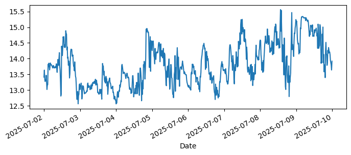
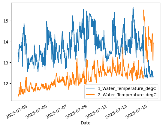
# Plot temperature from upper (1-meter) and lower (10-meter) sensors
aqua['1_Water_Temperature_degC'].plot()  # 1-meter
aqua['2_Water_Temperature_degC'].plot()  # 10-meter
plt.legend()

<matplotlib.legend.Legend at 0x791ff85e8450>

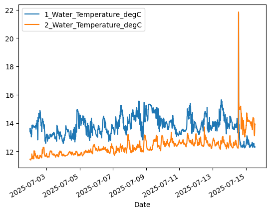
Note the spike in the temperature data on July 14, and then the apparent switch of the Sensor 1 and Sensor 2 data streams. What do you think happened at the Aquarium?

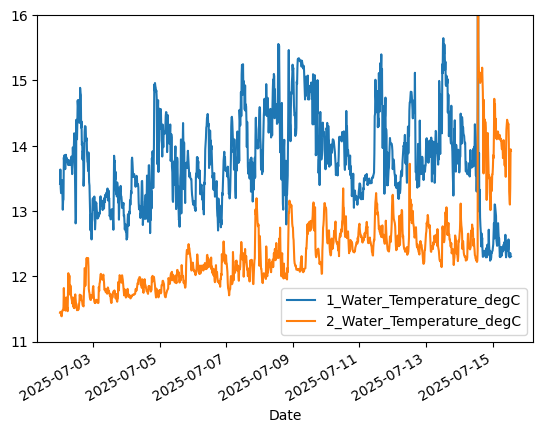
We’ll learn how to use boolean indexing to mask out bad data later. But for now, let’s change the y-axis limits to zoom in on the good data.

# Plot temperature from upper (1-meter) sensor
aqua['1_Water_Temperature_degC'].plot()
aqua['2_Water_Temperature_degC'].plot()
plt.ylim([11.0,16.0])   # Set y-axis limits to ignore data spike
plt.legend()

<matplotlib.legend.Legend at 0x791ff85a4c50>

Using timeseries capabilities

We can take advantage of built-in datetime functionality in Pandas to examine data at aggregated time intervals, like daily; and to examine diurnal variability (within each day).

First let’s examine the DataFrame index:

# The DataFrame index has a numpy "datetime64[ns]" data type
aqua.index

DatetimeIndex(['2025-07-02 00:00:00', '2025-07-02 00:15:00',
               '2025-07-02 00:30:00', '2025-07-02 00:45:00',
               '2025-07-02 01:00:00', '2025-07-02 01:15:00',
               '2025-07-02 01:30:00', '2025-07-02 01:45:00',
               '2025-07-02 02:00:00', '2025-07-02 02:15:00',
               ...
               '2025-07-15 11:00:00', '2025-07-15 11:15:00',
               '2025-07-15 11:30:00', '2025-07-15 11:45:00',
               '2025-07-15 12:00:00', '2025-07-15 12:15:00',
               '2025-07-15 12:30:00', '2025-07-15 12:45:00',
               '2025-07-15 13:00:00', '2025-07-15 13:15:00'],
              dtype='datetime64[ns]', name='Date', length=1298, freq=None)

# Extract the date from each datetime value in the index using the .date property
aqua.index.date

array([datetime.date(2025, 7, 2), datetime.date(2025, 7, 2),
       datetime.date(2025, 7, 2), ..., datetime.date(2025, 7, 15),
       datetime.date(2025, 7, 15), datetime.date(2025, 7, 15)],
      dtype=object)

We can use .resample() to resample the DataFrame over a specific time resolution (“1D” = 1 day), returning the minimum (.min()) and maximum (.max()) values at the resampled resolution:

aqua_dailymin = aqua.resample("1D", origin='start_day').min()
aqua_dailymax = aqua.resample("1D", origin='start_day').max()

We now have DataFrames with just one record (row) per day!

aqua_dailymin

	1_Depth_m	Qual_1_Depth	2_Depth_m	Qual_2_Depth	1_Water_Temperature_degC	Qual_1_Water_Temperature	2_Water_Temperature_degC	Qual_2_Water_Temperature	1_Salinity_PSU	Qual_1_Salinity	...	Qual_2_Sonde_pH	1_Density_kg/m^3	Qual_1_Water_Density	2_Density_kg/m^3	Qual_2_Water_Density	1_Sonde_Batt_V	2_Sonde_Batt_V	Logger_Batt_V	1_Sonde_ID	2_Sonde_ID
Date
2025-07-02	0.804	210	9.769	210	12.565	210	11.388	210	27.520	210	...	210	1020.44613	210	1022.25050	210	11.7	13.8	13.0	NaN	NaN
2025-07-03	0.862	210	9.816	210	12.683	210	11.590	210	28.036	210	...	210	1020.95768	210	1022.39893	210	11.7	13.8	13.0	NaN	NaN
2025-07-04	0.882	210	9.839	210	12.563	210	11.662	210	27.327	210	...	210	1020.31357	210	1022.34168	210	11.6	13.8	13.0	NaN	NaN
2025-07-05	0.976	210	9.925	210	12.759	210	11.680	210	24.558	210	...	210	1018.04794	210	1022.19333	210	11.3	13.8	13.0	NaN	NaN
2025-07-06	0.912	210	9.872	210	12.702	210	11.840	210	27.261	210	...	210	1020.12523	210	1022.28316	210	11.5	13.8	13.0	NaN	NaN
2025-07-07	0.955	210	9.889	210	13.146	210	11.709	210	27.778	210	...	210	1020.39621	210	1022.06330	210	11.5	13.8	13.0	NaN	NaN
2025-07-08	0.913	210	9.869	210	12.795	210	11.896	210	27.748	210	...	210	1020.40477	210	1021.99987	210	11.5	13.8	13.0	NaN	NaN
2025-07-09	0.926	210	9.902	210	13.398	210	12.038	210	27.377	210	...	210	1020.06360	210	1022.05351	210	11.5	13.8	13.0	NaN	NaN
2025-07-10	0.923	210	9.878	210	13.050	210	12.309	210	27.690	210	...	210	1020.53203	210	1021.83855	210	11.2	13.8	13.0	NaN	NaN
2025-07-11	0.840	210	9.804	210	13.180	210	12.318	210	27.572	210	...	210	1020.30141	210	1021.94333	210	11.5	13.8	13.0	NaN	NaN
2025-07-12	0.923	210	9.875	210	13.189	210	12.191	210	28.267	210	...	210	1020.82972	210	1021.82511	210	11.2	13.8	13.0	NaN	NaN
2025-07-13	0.858	210	9.804	210	13.237	210	12.141	210	27.482	210	...	210	1020.05341	210	1022.25472	210	11.5	13.8	13.0	NaN	NaN
2025-07-14	-0.010	210	-0.011	210	12.240	210	12.220	210	0.013	210	...	210	1021.38435	210	1020.60829	210	11.5	13.3	13.0	NaN	NaN
2025-07-15	9.642	330	0.716	330	12.291	210	13.099	210	29.540	210	...	210	1022.19247	330	1020.99987	330	12.0	13.4	13.0	NaN	NaN

14 rows × 39 columns

Look at the large changes in depth for the two sensors, 1_Depth_m and 2_Depth_m, starting on July 14!

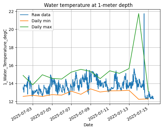
Use the resampled daily DataFrames to plot the 1-meter daily minimum and maximum on top of the raw data at the original 15-minute resolution.

aqua['1_Water_Temperature_degC'].plot(label="Raw data")
aqua_dailymin['1_Water_Temperature_degC'].plot(label="Daily min")
aqua_dailymax['1_Water_Temperature_degC'].plot(label="Daily max")
plt.legend()
plt.ylabel("1_Water_Temperature_degC")
plt.title("Water temperature at 1-meter depth")
plt.grid()

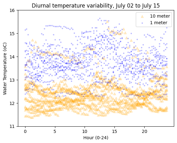
Now let’s focus on how temperature varies throughout the day (“diurnally”). First, use the DataFrame index to create an array of time values as fractional hours. For example, 12:30 is 12.5. We use the .hour and .minute properties:

hours_minutes = aqua.index.hour + aqua.index.minute / 60

hours_minutes

Index([  0.0,  0.25,   0.5,  0.75,   1.0,  1.25,   1.5,  1.75,   2.0,  2.25,
       ...
        11.0, 11.25,  11.5, 11.75,  12.0, 12.25,  12.5, 12.75,  13.0, 13.25],
      dtype='float64', name='Date', length=1298)

# Plot temperature as a scatter plot
plt.scatter(
    hours_minutes, aqua['2_Water_Temperature_degC'], label='10 meter',
    s=30, c='orange', marker='^', alpha=0.2
)
plt.scatter(
    hours_minutes, aqua['1_Water_Temperature_degC'], label='1 meter',
    s=5, c='blue', marker='o', alpha=0.2
)
plt.ylim([11.0,16.0])   # Set y-axis limits to ignore data spike
plt.xlabel("Hour (0-24)")
plt.ylabel("Water Temperature (oC)")
plt.legend()
plt.title(
    f"Diurnal temperature variability, {aqua.index.min():%B %d} to {aqua.index.max():%B %d}"
);

In the title, we used datetime formatting codes with f string formatting. See https://strftime.org and https://www.strfti.me. Here’s a simpler example:

f"{aqua.index.min():%B %d}"

'July 02'

The slice() function can be convenient for generating indices over an interval. The syntax is:

slice(start, stop, step=None)

For example, we can apply a slice on the timeseries DataFrame index to plot 1-meter temperature from the start of the timeseries to July 9. Notice that we use None to start at the beginning of the time series and can define a date as a string!

aqua['1_Water_Temperature_degC'].loc[slice(None, '2025-07-09')].plot(
    label="Raw data", figsize=(8,3)
);

Try exploring the data

Can you answer some of the following questions by making plots and using the functions you already know?

• What was the warmest ocean temperature seen in this data? (Feel free to slice the data to ignore periods of seemingly incorrect measurements.)

• On average, how much colder is the deep (10-meter) sensor than the shallow (1-meter) sensor? (Feel free to slice the data to ignore periods of seemingly incorrect measurements.)

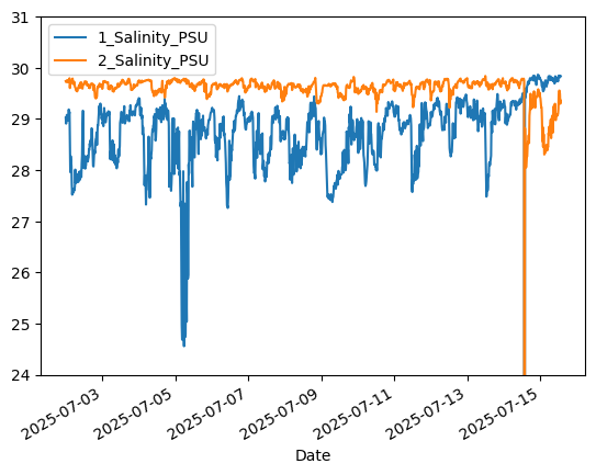
• What day likely had a significant rain event? (Hint: rain is fresh water, and the ocean is salty.)

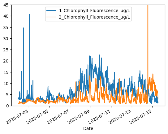
• What direction is phytoplankton growth trending in over this data period? (Hint: chlorophyll concentration is a measure of how much phytoplankton are in seawater.)

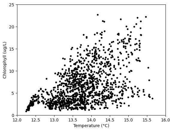
• What is the relationship between near-surface ocean temperature and phytoplankton?

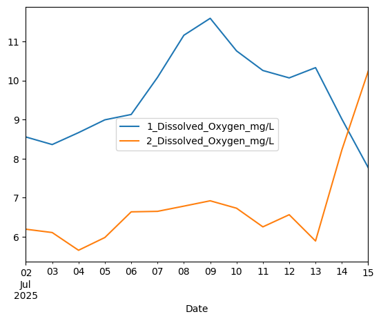
• Can you plot the mean daily oxygen concentration at 1- and 10-meter depths (the two Dissolved_Oxygen_mg/L columns)?

# Warmest ocean temperature
# Note: we are using .loc[slice()] to slice the data in time
# to ignore bad data from July 13 onwards
print(aqua['1_Water_Temperature_degC'].loc[slice(None,'2025-07-13')].max())
print(aqua['2_Water_Temperature_degC'].loc[slice(None,'2025-07-13')].max())

15.648
13.724

# Average temperature difference between shallow and deep sensors
# Note: we are using .loc[slice()] to slice the data in time
# to ignore bad data from July 13 onwards
print(aqua['1_Water_Temperature_degC'].loc[slice(None,'2025-07-13')].mean() -
      aqua['2_Water_Temperature_degC'].loc[slice(None,'2025-07-13')].mean())

1.6307517421602782

# Phytoplankton growth trend appears to be initially upwards, then downwards after July 9
aqua['1_Chlorophyll_Fluorescence_ug/L'].plot()
aqua['2_Chlorophyll_Fluorescence_ug/L'].plot()
plt.ylim([0.0,45.0])  # Crop y-limits due to data spike
plt.legend()

<matplotlib.legend.Legend at 0x791ff8301290>

# Ocean salinity reveals a freshening signal on 7/5/25, likely from rain
aqua['1_Salinity_PSU'].plot()
aqua['2_Salinity_PSU'].plot()
plt.ylim([24,31])  # Crop y-limits due to data spike
plt.legend()

<matplotlib.legend.Legend at 0x791ff820f210>

# Relationship between temperature and chlorophyll
# (The amount of phytoplankton seems to increase with warmer
#  near-surface temperatures!)
plt.scatter(aqua['1_Water_Temperature_degC'],
            aqua['1_Chlorophyll_Fluorescence_ug/L'],
            c='k',s=10)
plt.xlim([12.0,16.0])   # Crop axis limits due to incorrect data
plt.ylim([0.0,25.0])
plt.xlabel('Temperature (°C)')
plt.ylabel('Chlorophyll (ug/L)')

Text(0, 0.5, 'Chlorophyll (ug/L)')

# Mean daily oxygen at 1 and 10 meters
aqua_dailymean = aqua.resample("1D", origin='start_day').mean()
aqua_dailymean[['1_Dissolved_Oxygen_mg/L', '2_Dissolved_Oxygen_mg/L']].plot()

<Axes: xlabel='Date'>

Part 3: Logical operations

Often, we will want to compare two numbers or variables. We do this using the following logical operations:

• == : equal

• != : not equal

• > : greater than

• >= : greater than or equal to

• < : less than

• <= : less than or equal to

• and or & : are both booleans true?

• or or | : is either boolean true?

• not or ~ : reverse the boolean (True -> False, False -> True)

• in : is a member

• not in : is not a member

Each logical operation evaluates to (returns) a boolean — True or False. Consider the following examples:

3 == 3

True

3 == 3.0    # integers can be compared to floating-point numbers

True

not 3 == 3

False

3 == 5

False

3 != 5

True

3 > 5

False

5 <= 5

True

(3 != 5) or (3 > 5)

True

(3 != 5) and (3 > 5)

False

Applying a logical comparison to a NumPy array gives a boolean array!

x = np.array([1,2,3,4,5,6])

print(x < 4)
print(x <= 4)

[ True  True  True False False False]
[ True  True  True  True False False]

# Note: "not" can't be applied to an entire boolean array.
# Instead, we have to use "~":
print(~np.array([True, False, True]))

[False  True False]

Note that membership tests work on lists, arrays, and strings:

print(3 in x)      # this is asking: "is 3 in x?"

True

print(7 in x)

False

print(3 not in x)  # this is asking: "is 3 not in x?"

False

print('o w' in 'hello world')

True

print('World' in 'hello world')   # note that string membership is case-sensitive

False

Heads up: this next skill is super powerful. We saw above that applying a logical comparison to an array of numbers gives us a boolean array.

We can use boolean arrays as “masks” to select certain elements of an array. This is called boolean indexing.

Here are a few ways to use it:

# Here are the pH values from last week's lesson:
pH_measurements = np.array([7.84, 7.91, 8.05, np.nan, 7.96, 8.03])
print('pH measurements:', pH_measurements)

# Remember that we can test for missing data (np.NaN values) using np.isnan():
print('Result of np.isnan():', np.isnan(pH_measurements))

# The resulting boolean array can be used to extract only the valid data:
print('Array after removing missing data:', pH_measurements[~np.isnan(pH_measurements)])

pH measurements: [7.84 7.91 8.05  nan 7.96 8.03]
Result of np.isnan(): [False False False  True False False]
Array after removing missing data: [7.84 7.91 8.05 7.96 8.03]

# Let's revisit the Seattle temperatures from earlier:
seattle_temps = np.array([40.0,40.6,44.2,48.4,54.9,60.2,66.2,66.7,60.5,52.0,44.5,39.6])

# Applying a logical comparison creates a boolean array, or "mask":
print(seattle_temps > 60)

[False False False False False  True  True  True  True False False False]

# Now let's use the mask to retrieve only the elements where the mask is True:
seattle_temps[seattle_temps > 60]

# Note: this only works when the mask is the same length as the array!

array([60.2, 66.2, 66.7, 60.5])

# The boolean indexing gives the same result as specifying the actual array indices:
seattle_temps[[5,6,7,8]]

array([60.2, 66.2, 66.7, 60.5])

We can use boolean indexing to handle the data outlier in the Seattle Aquarium time series! Let’s apply the threshold of 16°C we used earlier to set values as “missing”, np.nan. To do this, we’ll use the extended .loc[] syntax to assign a value to a column based on a criteria:

dataframe.loc[BOOLEAN_ARRAY, COLUMN_NAME] = NEW_VALUE

aqua.loc[aqua['1_Water_Temperature_degC'] > 16, '1_Water_Temperature_degC'] = np.nan
aqua.loc[aqua['2_Water_Temperature_degC'] > 16, '2_Water_Temperature_degC'] = np.nan

Now redo the plot we did earlier. No need to clip the y axis range anymore! But the data still seem to switchover between the two sensors …

aqua['1_Water_Temperature_degC'].plot()  # 1-meter
aqua['2_Water_Temperature_degC'].plot()  # 10-meter
plt.legend()

<matplotlib.legend.Legend at 0x791ff8314dd0>

How many months of the year is Seattle 40°F or colder? Try using boolean indexing and a function that you’ve learned to calculate and print the answer:

# Write your code here:
len(seattle_temps[seattle_temps > 40])

10